The APyT reconstruction command line script
Reconstruction of atom probe data in APyT follows the conventional projection scheme described by Bas et al. Two reconstruction modules are available:
Classic scheme — The tip radius is derived dynamically from the applied voltage.
Taper geometry — The tip geometry is predefined by a taper angle and an initial radius.
Note
This script performs only the essential three-dimensional reconstruction and basic visualization. The resulting atomic positions are exported to an ASCII text file, which can then be used for further analysis and visualization.
Invoking the command line script
The script apyt_reconstruction is installed automatically when following the
installation instructions. It requires a single positional
argument (the measurement ID in the database). Several optional arguments are
also available. For a full list, run:
apyt_reconstruction --help
Commonly used options include:
--no-sql— Skip connecting to an SQL database. Instead, load measurement data and metadata from a local database. This is the typical mode for local testing or standalone workflows.--cache— Load measurement data from a binary NumPy.npyfile in the working directory. This avoids repeated file parsing or database queries, significantly speeding up subsequent runs.Note
The cache file is created automatically on the first run and reused for subsequent runs on the same measurement ID.
Note
This option only takes effect when the measurement data is retrieved from the SQL database.
--module <classic|taper>— Choose which reconstruction module to use. Defaults totaper.
A typical invocation might look like:
apyt_reconstruction --no-sql --module classic 1
Graphical user interface
Running apyt_reconstruction opens a graphical interface for interactive
adjustment of the reconstruction parameters. The examples below show a tungsten
reference measurement reconstructed with both the classic and taper module:
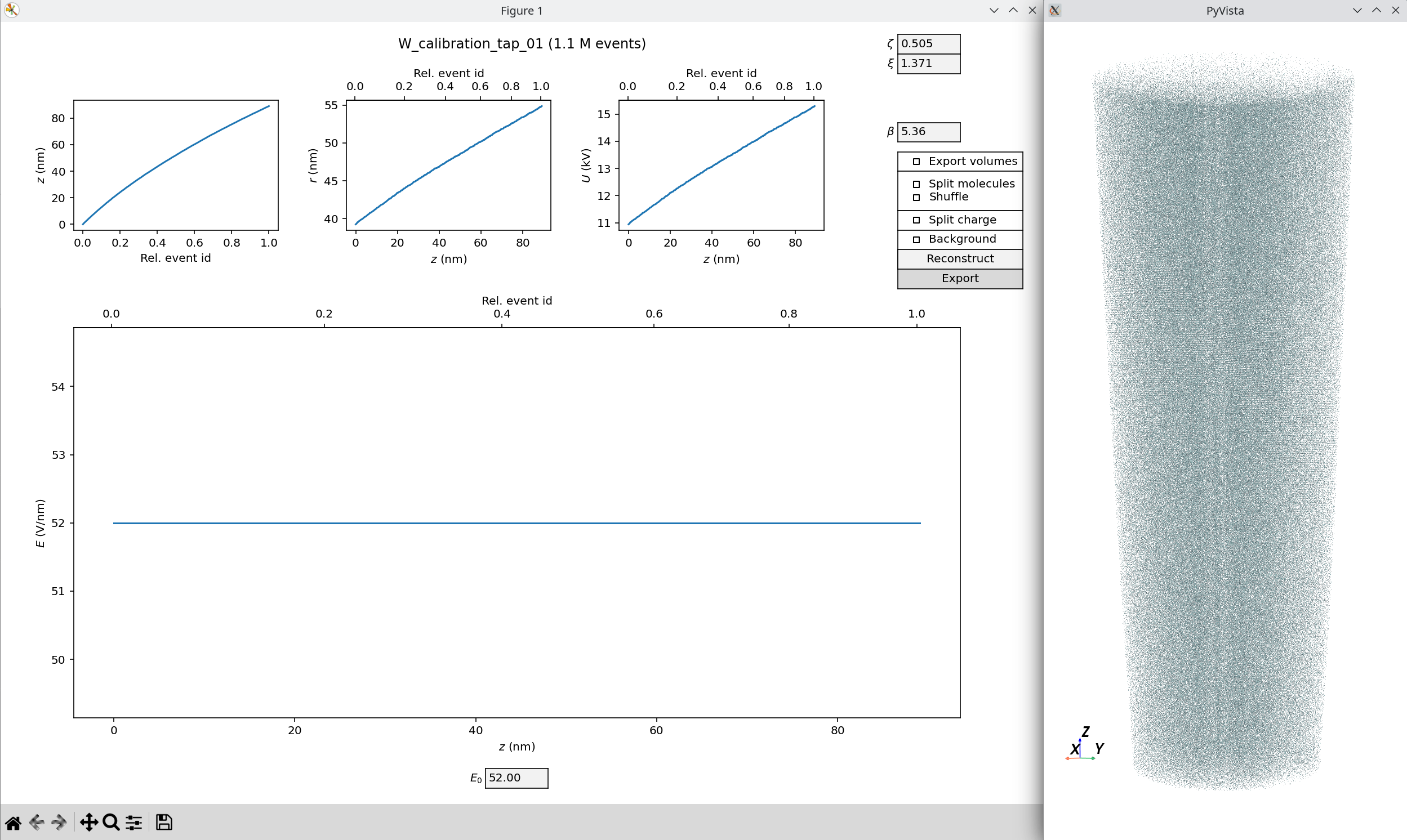
Reconstruction of a tungsten measurement using the classic module.

Reconstruction of a tungsten measurement using the taper geometry module.
The graphical interface is divided into three main parts:
Bottom panel — Shows the evolution of the evaporation field \(E\) as a function of the tip depth position \(z\) (bottom axis) and relative to the number of reconstructed events (top axis).
Note
In the classic module, the evaporation field is a constant defined by the value in the \(E_0\) field.
Top row — Displays the evolution of tip depth position \(z\), tip radius \(r\), and applied voltage \(U\).
Right panel — Provides various reconstruction parameters and export options. The Reconstruct button triggers the reconstruction, while Export writes the reconstructed tip positions to an ASCII xyz file format. A basic visualization of the reconstructed tip is provided via PyVista (see figures from above).
Reconstruction parameters
Several free parameters need to be adjusted properly for a correct reconstruction:
\(\zeta\) — Detector efficiency.
\(\xi\) — Image compression factor of the device.
\(r_0\) — Initial tip radius (only active in taper geometry).
\(\alpha\) — (Full) taper angle (only active in taper geometry).
\(\beta\) — Field factor.
Export options
Several export options are available for the reconstructed 3D tip positions:
Export volumes — Add an additional column to the output file with the reconstructed event volumes.
Split molecules / Shuffle — Split molecules into their constituent atoms, all placed at the same position. The Shuffle option randomizes the order of atoms within each molecule in the output file.
Split charge — Export different charge states with different IDs (see console output for the chemical mapping to IDs).
Background — Also export background atoms (always labeled with ID zero).
Taper geometry
When using the taper geometry module, reconstruction parameter adjustment is partially automated. If any of the parameters \((r_0, \alpha, \beta)\) is known (e.g. taper angle \(\alpha\) from specimen preparation), it can be marked as fixed (see corresponding figure). The two remaining parameters are then automatically adjusted to maintain a constant evaporation field \(E_0\) in the bottom panel.
The measurement range for this adjustment can be chosen using the min and max fields in the bottom, as indicated by the vertical dashed lines in the evaporation field plot.
Database upload
Upon closing the graphical interface, the user is asked whether the final reconstruction parameters should be uploaded to the database.
See also
For further technical details, see the reconstruction module.